Introduction
Finesse is a simulation program for interferometers. The user can
build any kind of virtual interferometer.KAT file, Finesse input text file
describing the interferometer in the form of components and connecting
nodes. The purpose of this document is to review and motivate the
parameters in the file, as well as to keep track of changes in the
file.IFO Matching
As from TDR
(VIR–0128A–12), the
required values for PR and SR radius of curvature (RoC) is
\(1430.0\) m, both the PRC and the SRC are marginally stable for
that value. The actual measured values for PRM and SRM are
\(1477.1\) m
(VIR-0029A-15) and
\(1443.35\) m
(VIR-0028A-15),
respectively. In the KAT file the RoCs are set to the design value
(\(1430.0\) m) and the compensation plates (CP) focal length is such
that the PRC and SRC are well matched to the arm cavities, even though
this requires a divergent compensation plate
(VIR-0629A-18).
Update
December 7, 2021 - the focal length of the CPs have been further optimised to mode match the recycling cavities to the arm cavities.
The OMC modelling
Finesse |
\(1100\) |
FSR |
\(834\) MHz |
\(T_{In}\) |
\(0.285\)% |
\(T_{Out}\) |
\(0.285\)% |
\(T_{HR1}\) |
\(1.1\)ppm |
\(T_{HR2}\) |
\(1.3\)ppm |
Throughout |
\(\approx2\%\) |
Loss 1 |
\(60\)ppm |
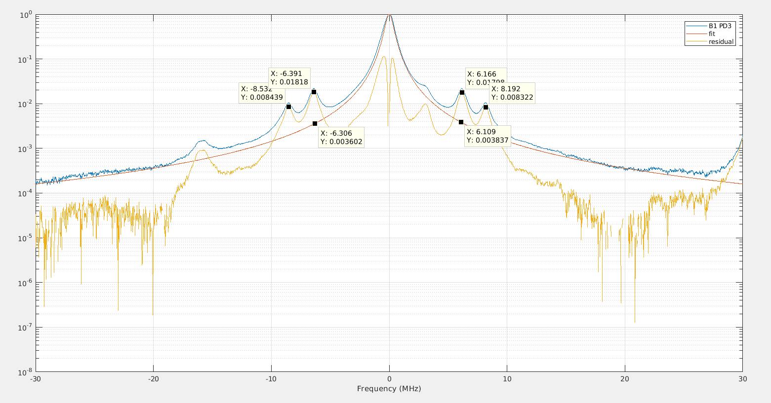
Fig. 1 Matching tails between the Airy’s curve and the real data plot.
\[\mathcal{F}\approx \frac{\pi}{1-r_1r_2r_3r_4} \]Where all the \(r\) are amplitude reflectivities. Here \(r_1\) is taken equal to \(r_2\); them refers respectively to the input and output mirrors. Following \(r_3\) refers to the HR curved mirror and \(r_4\) refers to the flat HR mirror. Setting \(r_3\approx 1\) (ideal HR mirror) and \(r_4=1-L-t_4\), were L is the cavity round trip loss and \(t_4\) is the amplitude transmissivity of the second HR mirror. Computing the formula we find the transmissivities in power mentioned in Table 1. The 60ppm round trip losses measured in the cavity come from various types of scattering and absorption in the coating and in the substrate of the cavity; it roughly match the measured throughput.
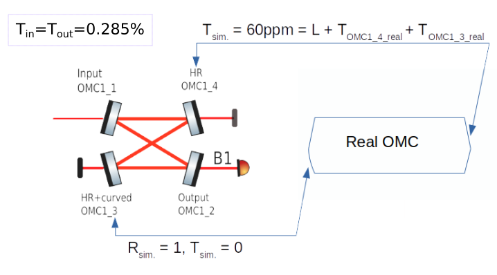
Fig. 2 Visual representation of the losses used in the simulation.
Finesse |
\(1089.29\) |
FSR |
\(834.569\) MHz |
Throughout |
0.979 |
Loss 2 |
\(0.006\) |
We have chosen to keep the round trip loss number round in the simulation, this lead to a little discrepancy between the measured Finesse and the simulated one. However that doesn’t affect the overall work of the simulated OMC, if it will be required in future the Finesse values can be made equal.
Arms characterization
The arm lengths of the IFO are been measured with a FINESSE simulation, the full code is in Arms characterization.
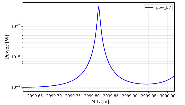
Fig. 3 Simulation result of the North arm’s measurement.
\[\begin{aligned} North\,\,arm:\, & 0.4528\times FSR\\ West\,\,arm:\, & 0.4416 \times FSR\,\,. \end{aligned}\]Knowing that:
\[f_{56MHz}=56436993MHz\,\,\, \text{and}\,\,\, FSR=\frac{c}{2L} \]We can then compute the arm lengths in few simple steps.
\[f = n\times FSR + \Delta f\\ \]\[56436993 MHz= n\times FSR + 0.4528\times FSR\,\,. \]The closest round number \(n\) that fit the equation is \(1129\), this lead to:
\[FSR=\frac{56436993MHz}{1129 + 0.4528}\,\,, \]so we have:
\[MMT L_{North} = \frac{c}{2FSR}=2999.818m\,\,.\]The same procedure it’s been done for the West Arms. It leads to \(L_{West}=2999.788\), VIR-1080A-21.
EOMs modulation depths
The EOMs installed in Ad.Virgo+ are phase modulators. Each of them requires an amplifier that gives power to the crystal that form the EOM; in order to create the phase shift in the side bands. For the one that produce the \(56\) MHz sideband the amplifier of \(1\) W was replaced by one of \(2\) W. This change lead to an electric signal ampitude of \(0.12\) dBm applied on the EOM, It can be monitorized using INJ_LNFS_AMPL\(1\)/\(2\)/\(3\) channels. The corrisponding frequencies channels are INJ_LNFS_FREQ\(1\)/\(2\)/\(3\). The change was made in order to increase the modulation depth from \(0.16\) rad to \(0.25\) rad, since the SNR value was too small to gain a good error signal (LB \(38123\)).
Focal lengths optimisation for OMC’s mode-matching
The new parameters for the OMC in Ad.Virgo+ provided some mode mismatch inside the Virgo kat script, specifically on the first beam splitter (OMC:math:1_\(1\)) that compose the OMC cavity. The mode match in the rest of the cavity is provided by the command ‘cav‘ that defines the cavity. To fix this problem it’s been made a simulation to minimise the mode mismatch between OMC\(1\)_\(1\) and the two lenses that serve to mode match it, MMT_L\(1\) and MMT_L\(2\). A ‘mmd‘ detector is been used to simultaneously scan on the two focal lengths. We reached a mode mismatch \(\sim 10^6\), this is enough to confirm that the OMC is in mode-match state, since at this point the variation on the focal lengths of the lenses is so negletable that is not manually possible anymore.
Coating and substrate diameters for Ad.Virgo+, Phase I
We report here the tables of the designed values with the coating and substrate diameters used in Ad.Virgo+, Phase I (Ref \(VIR-0128A-12\)). To stay updated with the most recent changes, you can see the Virgo wiki.
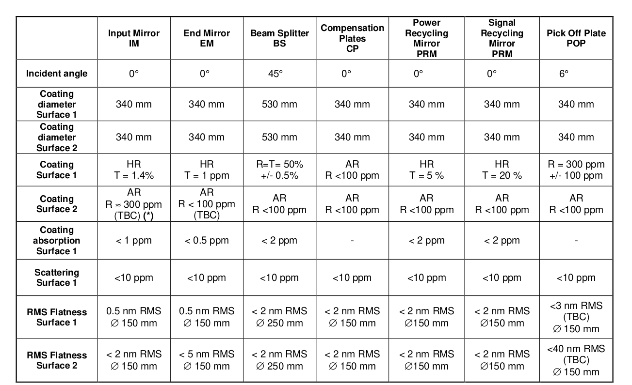
Fig. 4 A summary of the coatings main features of the Ad.Virgo+ (Phase I) mirrors at 1064 nm.
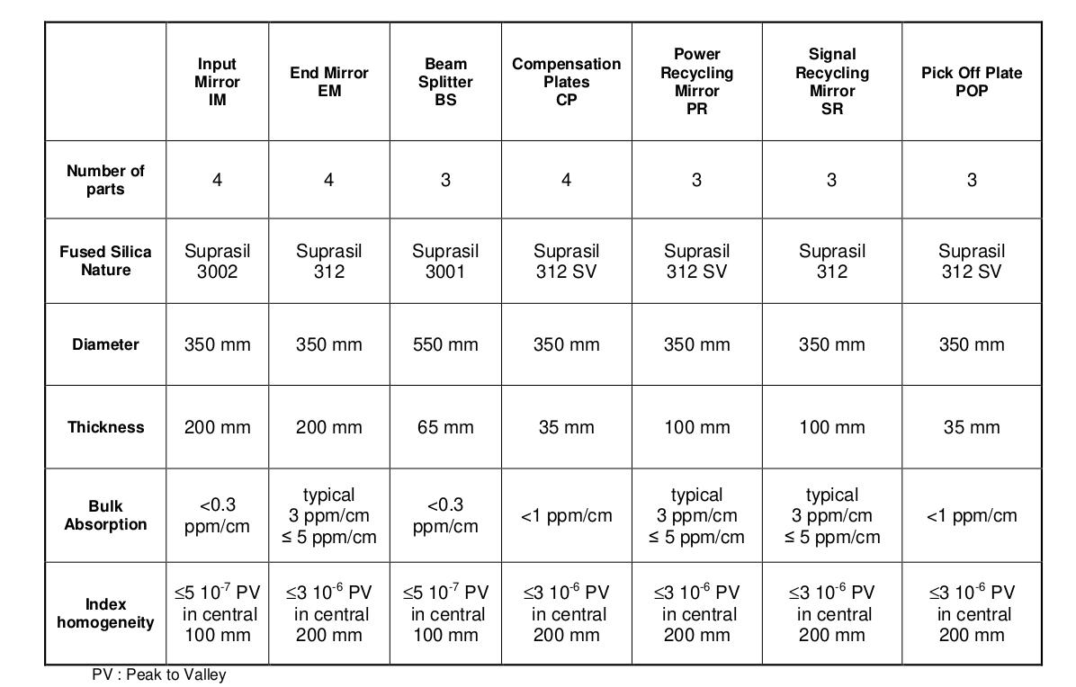
Fig. 5 Specifications of the bulk substrates for the Ad.Virgo+ (Phase I) mirrors.
Using the KatScript
Pretuning the model
We bring the model to a sensible configuration by “pretuning”, which used the power of the carrier (main laser beam without RF modulation) to set the desired resonance conditions.
This is done using following steps:
Switch off the modulators to only use main carrier field in the following steps.
Remove the SR and PR mirrors. This is to remove any cross-coupling between the two arms, so we can tune them independently from each other.
Move the arm cavity end mirrors to maximise power in each arm so the arm cavities are on resonance.
Move the arm cavities to minimise power at the output so the interferometer is at the dark fringe
Restore the PR mirror, and move it to maximise power in the PRC so the PRC is on resonance.
Restore the 56MHz modulator.
Restore the SR mirror, and move it to maximise power in B4_112MHz.
Restore the other modulators.
#TODO: add a comparison plot between the old and new pre-tuning strategies.
Update 21/05/2022 - Riccardo
Updated the common kat to add the followings: 1) The RoC of the PRM and SRM are set to the measured values. 2) The CPs’ focal length has been tuned accordingly 3) The recycling cavities are defined as “long cavities”
The CP’s focal length comes from VIR-0641A-22
Behavior of beam parameters in the PRC
This section illustrates the behavior of the beam parameter in the PRC when defining the cavity as “short” or “long” by including or excluding the arms.
The following plots were generated using a simplified model of the three mirror coupled cavity including the PRC and one of the arm cavities.
Fig. 6 An overview of the behavior of the beam parameter seen through the power in the PRC.
Fig. 7 The short cavity with fixed q converges to the long cavity with increased maxtem.
Fig. 8 The short cavity has a mismatch at the ITM whereas the long cavity does not.
Fig. 9 The waist size at the laser varies greatly when defining the short cavity.
Fig. 10 The waist position at the laser varies greatly when defining the short cavity.